


A prototype can correctly predict 92% of cases and never be used. At 78% accuracy, a simpler approach can reduce stockouts if its errors are understood, its recommendations arrive in time and managers know when not to follow them.
The best score is not always the best product.
Data science answers several kinds of question: what happened, why it happened, what is likely to happen, what would happen if a different action were taken, and which decision best respects the constraints? Confusing these questions leads teams to use prediction where an experiment or a rule would have been more useful.
1. Key figures: the model is only a small part of the system
A Google Research study based on interviews with 53 AI practitioners in several countries observed "data cascades" among 92% of participants. These problems, triggered by insufficient data practices, produced cumulative downstream effects, often late and difficult to see. The figure does not measure all enterprises, but it documents the frequency of the phenomenon in high-stakes projects.
Google also describes its data validation system used by hundreds of product teams on several petabytes a day. The authors insist on deceptive behaviour: a machine-learning pipeline can continue to run with an unexpected schema, abnormal distribution, or a mismatch between training and production data.
The same research group’s “ML Test Score” framework sets out 28 tests and monitoring requirements across data, features, models and infrastructure. That breadth gives a more realistic view of production readiness than accuracy alone.
Forecasting competitions offer another lesson. M4 compared 61 methods across 100,000 time series. Of the 17 most accurate approaches, 12 combined several methods. The hybrid winner, which blended exponential smoothing with a neural network, was nearly 10% more accurate than the selected combination benchmark. In this setting, all six “pure” machine-learning methods underperformed that benchmark. Sophistication does not automatically beat a strong statistical baseline.
Finally, a probability score is not necessarily a reliable probability. The scikit-learn documentation notes that, in a well-calibrated classifier, approximately 80% of cases assigned a score close to 0.8 should actually belong to the positive class. A model can rank cases correctly while remaining overconfident; that distinction affects decision thresholds and costs.
2. The decision contract
Every project starts with a short contract between business, data and operations. It does not describe the algorithm. It describes the decision.
| Field | Example: anticipate the risk of a late order |
|---|---|
| Decision | contact, accelerate or do nothing |
| Moment | 48 hours before the promised date |
| Population | open orders with confirmed transport |
| Observed result | delay exceeding 24 hours |
| Horizon | two days |
| Possible action | customer message or change of carrier |
| False positive cost | unnecessary call and operational overload |
| False negative cost | dissatisfaction, penalty, churn |
| Capacity | 500 cases processed per day |
| Success criterion | net reduction in delays and complaints |
| Fallback | current business rule |
No value is created unless the decision changes. Predicting that an order will arrive late after its final dispatch produces interesting information, but nothing that can be acted upon.
The contract also defines operational capacity. If the team can process only 500 cases, optimising accuracy across the full dataset is less useful than ranking the first 500 correctly.
3. Six families of questions, six methods
3.1. Describe
Descriptive statistics measure volumes, distributions, cohorts and trends. They answer: “What happened?” Many decisions can already be improved through sound segmentation and interval estimates, without a predictive model.
3.2. Diagnose
Diagnostic analysis seeks factors associated with a change. It uses decomposition, journey analysis, regression and domain knowledge. Association does not prove causation, but it narrows the field of investigation.
3.3. Predict
Prediction estimates an unknown outcome: demand, churn, default or delay. It requires a defined horizon, observable ground truth and out-of-sample evaluation. Its quality depends on the decision context.
3.4. Estimate a causal effect
Causal analysis asks what would have happened without the action. A randomised test is often the benchmark; quasi-experimental methods can help when randomisation is impossible. A churn model predicts who is likely to leave. An uplift model identifies who will stay because of an intervention. They are not necessarily the same customers.
3.5. Optimise
Optimisation selects an action under constraints such as inventory, capacity, time, risk and fairness. It can use forecasts as inputs. A better forecast will not improve the outcome if the optimiser or business process cannot act on it.
3.6. Detect anomalies
Anomaly detection flags deviations such as fraud, equipment failure and corrupted data. It often operates with few labelled examples, making alert rate and investigation cost central metrics.
Framing selects the question family before the technique. Asking for “an AI model” short-circuits that essential choice.
4. The baseline: the competitor the model must beat
A baseline may be the average, the latest value, an expert rule or the existing human process. It must be measured honestly over the same period and population.
For a weekly forecast, “the same week last year, adjusted for trend” can be surprisingly hard to beat. For churn, “contact accounts that have not logged in for thirty days” can capture much of the value. If a complex model gains only 0.5 points but requires substantial infrastructure, the rule remains preferable.
Current costs must also be measured: how many decisions are made, how much time they take, which errors occur and which opportunities are missed? This baseline is used to calculate net value, not just statistical performance.
The baseline remains available in production as a fallback. A system that cannot revert to a simple rule during an incident is fragile.
5. Data: building ground truth
The target variable represents the outcome to be learned. Defining it deserves as much attention as designing the model.
A “lost customer” may mean cancellation, no purchase for 90 days or failure to renew a contract. These definitions create different populations. The label must be observable after the prediction horizon and stable over time.
The collection follows four principles.
Representativeness. The dataset must cover the relevant seasons, channels, regions, products and rare cases. A sample drawn from the most active customers often overestimates performance.
Temporal validity. A training variable must be available at the actual time of the decision. Incorporating the final status of a case into a feature creates target leakage.
Provenance. Each variable retains its source, formula, date and owner. Corrections are versioned.
Rights. Purpose limitation, data minimisation, retention, access and transparency are defined, especially for personal data.
A manual review of a few hundred records often reveals problems that code alone cannot expose: a repurposed business status, an inappropriate default value, missing events or inconsistent practices between teams.
6. Split training, validation and test data to reflect real-world conditions
A random split is not always appropriate. To predict the future, train on the past and test on a later period. To generalise to new customers, split by account. For images of the same object, closely related shots must remain in the same group.
Duplicates and near-duplicates are removed across datasets. Splitting near-identical photographs between two sets creates an illusion of generalisation.
The validation set is used to select parameters. The final test set remains hidden until selection is complete. Consulting it after every experiment gradually turns it into training data.
After launch, the time-based evaluation set is renewed. The world changes; a frozen test can remain reassuring even as real-world cases drift.
7. Choose the metric based on the cost of errors
Accuracy—the overall share of correct answers—is misleading when classes are imbalanced. If 1% of transactions are fraudulent, predicting “not fraud” in every case produces 99% accuracy and no value.
Recall measures the proportion of positive cases detected. Precision measures the proportion of alerts that are genuinely positive. Increasing one can reduce the other, so the threshold must reflect the operational trade-off.
For rankings, examine precision among the highest-ranked cases, lift and cumulative gain. For probabilities, measure discrimination and calibration. For forecasts, compare absolute error, relative error and performance across volume bands.
A cost matrix is even more concrete: euros, minutes, risks or capacity associated with each of the four outcomes. Evaluation should use the unit that matters to the decision.
Metrics must be segmented. An average can conceal poor performance in a region, on a new product or for a vulnerable population.
8. Calibration and thresholds: turning a score into a decision
A score of 0.8 is useful only if its meaning is known. A calibration curve compares predicted probabilities with observed frequencies. The Brier score and log loss provide aggregate measures, but scikit-learn emphasises that each combines several properties; the curve itself remains essential.
The threshold should not default to 0.5. It depends on capacity and costs. A team able to review 200 cases selects the 200 highest-risk cases, provided the ranking remains stable and the expected value is positive.
An abstention zone can be defined: act above one threshold, take no action below another, and require human review between the two. This structure is more honest than forcing a decision in every case.
Thresholds are versioned separately from the model. Operational capacity or costs may change without requiring retraining.
9. Explainability: provide actionable evidence
Global feature importance shows which factors generally influence the model. A local explanation shows what contributed to one specific score. Neither establishes causality.
Users need actionable evidence, such as “supplier delay above normal” or “three recent payment failures”, supported by the source data. A list of mathematical weights without context is not enough.
Explanations must also be tested for stability. If a small, immaterial variation radically changes the explanation, the interface must not present it as a definitive justification.
For consequential decisions, the explanation must also cover limitations, routes of recourse and the ability to correct underlying data. Transparency applies to the entire process.
10. From notebook to service
A notebook supports exploration; a production service must run repeatedly and reliably. Moving between the two requires several changes.
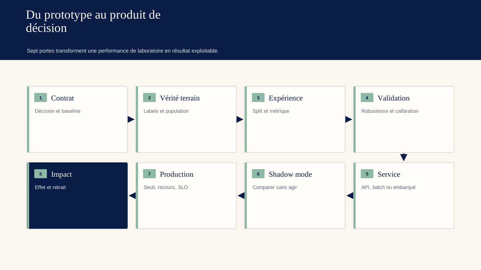
Data-preparation code becomes a tested pipeline. Dependencies are pinned. Data and parameters are versioned. Training is reproducible from a commit and a snapshot. The model is registered with its metrics and approvals.
Feature logic must be identical in training and serving. A calculation implemented differently in an API creates training-serving skew. Shared transformations, example-based tests and distribution checks reduce this risk.
The inference mode must follow the decision. Daily batch processing suits scheduled action lists. A real-time API suits an immediate response. Streaming is justified only when the cost of delay exceeds its operating cost.
Deployment begins in shadow mode: the model predicts without influencing decisions. Its outputs are compared with current practice while operational constraints are observed. Only then does a share of traffic or a pilot team begin using it.
11. Observability: data, model, system, decision
Four layers must be monitored.
Data. Schema, missing values, unknown categories, freshness, distributions and lineage.
Model. Scores, calibration, abstention rate, performance once labels arrive and stability by segment.
System. Availability, latency, errors, versions, cost and queues.
Decision. Adoption, workarounds, actions taken, business outcomes and adverse effects.
Data drift does not automatically imply a decline in performance, but it should trigger an investigation. Conversely, performance can deteriorate without obvious drift if the relationship between variables and outcomes changes.
Ground truth may arrive several months later. Early indicators can monitor coverage, scores, acceptance and input variables, but they must not be presented as substitutes for the final outcome.
Every alert needs an owner, a threshold and a defined response. If nobody knows what to do, monitoring creates anxiety rather than control.
12. Case study: prioritising sales outreach
A B2B company receives 12,000 leads per month. The sales team can contact 3,000 within 48 hours. The overall conversion-to-contract rate is 4%.
The prototype aims to predict contract signature. A simple baseline ranks leads by company size and form completeness. It achieves a 7% signature rate among the top 3,000.
The first model reaches 10%. Analysis, however, reveals leakage: the “scheduled appointment” variable, recorded after follow-up, appears in the training data. Once removed, performance falls to 8.5%. That is still better than the baseline, but the real gain is half the advertised figure.
Calibration also shows that the scores are overconfident. The team stops presenting them as percentages and uses priority bands instead. A control group retains the old rule. After eight weeks, the strategy increases net signatures by 12% within the team’s processing capacity, without slowing responses to small accounts.
The model is not deployed across all leads. Partner-sourced leads remain out of scope because their behaviour differs and the sample is too small. This limitation is a deliberate quality decision.
13. Productionise through stage gates
Before deployment, the project must pass a go/no-go gate review.
- Are decisions and actions defined?
- Are the baseline and current costs measured?
- Is the label available and dated?
- Do variables exist when deciding?
- Does the test reproduce the expected generalisation?
- Are the performances segmented and calibrated?
- Are critical errors and recourse defined?
- Is the pipeline reproducible and secure?
- Do the monitoring and fallback plans have clear owners?
- Will the value be measured by a credible pilot?
A “no” does not mean giving up; it identifies the next experiment. The gate protects production from pressure to show a result prematurely.
14. Total cost and value
Total cost includes extraction, annotation, experimentation, compute, platform, deployment, monitoring, human review and maintenance. The initial model may account for only a small fraction.
Expected value is calculated from decisions: number of actions × change in outcome × unit value, minus the cost of actions and errors. Uncertainty must also be included.
A pilot should estimate that change. An offline improvement is not enough if users ignore the score or customers respond differently in practice.
Maintenance costs must be budgeted. New categories, process changes, supplier updates and regulatory changes may require a new version. Without a long-term owner, the model becomes an orphaned asset.
15. Organisation: build a team around the decision product
The data scientist frames the problem, explores, models and evaluates. The data engineer makes the data reliable. The ML engineer industrialises the system. The business owner defines actions and costs. The product manager organises adoption. Legal and security teams frame the risks.
In a small team, one person may cover several functions. Independent review remains essential: the model’s author should not be its sole validator.
Data work must be planned and recognised. The study on cascades shows the consequences of a culture in which “everyone wants to work on the model, not on the data”. Correcting a definition or a source process can create more value than introducing a new algorithm.
16. A fourteen-week roadmap
Weeks 1 and 2 — Decision contract. Choose one decision, measure the baseline, document the costs and confirm the organisation can act.
Weeks 3 and 4 — Data. Define the label, audit the sources, search for leakage and build a time-based split.
Weeks 5 and 6 — Simple models. Test a rule, a linear model and a decision tree before trying more complex approaches. Compare performance across segments.
Weeks 7 and 8 — Decision design. Calibrate the model, select thresholds, simulate costs and capacity, and design explanations.
Weeks 9 and 10 — Production engineering. Build the pipeline, model registry, tests, API or batch job, logs and fallback.
Weeks 11 and 12 — Shadow mode. Observe real scores, latency, distributions and user responses without taking automated action.
Weeks 13 and 14 — Controlled pilot. Compare with a control group, measure outcomes and side effects, then decide whether to deploy, adapt or stop.
Discipline lies in the gates. Moving quickly does not mean skipping the evidence that distinguishes a demonstration from a product.
17. Frequently Asked Questions
17.1. How much data does it take?
The answer depends on signal strength, the number of variables, rarity and stability. A learning curve shows whether more examples still improve test performance. Quality and representativeness matter as much as volume.
17.2. Do you still need machine learning?
No. A rule, descriptive analysis, experiment or deterministic optimisation may answer the question better. Machine learning is useful when a generalisable pattern exists and leads to an actionable intervention.
17.3. How does this differ from predictive AI?
Predictive AI refers to systems that anticipate an outcome and incorporate it into a decision. Data science is broader, encompassing description, diagnosis, causality, experimentation, optimisation and the methodological lifecycle. The two overlap but are not synonymous.
17.4. When should you retrain the model?
Retrain when performance, data or processes move beyond defined thresholds, or on a justified schedule. Automatic weekly retraining can amplify an anomaly. Validation must precede promotion to production.
17.5. How should you explain a complex model?
Show the relevant factors, supporting source data, limitations and routes of recourse, then test the explanation for fidelity and stability. A visualisation does not turn correlation into causation.
18. What a data-science acceptance protocol can prove before deployment
Acceptance testing includes a business baseline, a time-based test set never used for training, minority segments and borderline cases. It compares average performance, calibration, error costs, stability and response time. An improvement in AUC is not enough if the operating threshold increases the most costly false rejections.
The shadow test runs predictions without influencing decisions. Teams compare recommendations with outcomes, measure the difference from the current rule and observe which data is genuinely available at the point of decision. This phase reveals temporal leakage that never appears in the notebook.
Before activation, the business owner understands why the threshold was chosen, the operations team can revert to the previous rule, security understands the data flows, support can explain errors, and the registry records the version, population, metrics, limitations, owner and review date. Together, these controls matter more than an isolated score because they show that the model produces a controllable decision in the real process, under load, with missing data and a route for correction.
After launch, a phased cohort limits exposure. Early results justify expansion only if value, fairness, reliability and operational burden remain within their guardrails.
The project record must also preserve rejected scenarios, abandoned variables, uncertainty intervals, human decisions that contradicted the recommendation and incidents during the cohort. A future review can then avoid selecting only favourable examples and distinguish lasting improvement from random variation, a population shift or exceptional intervention by the project team.
19. Logiks recommendations
Define the decision and its baseline before opening a notebook. Make the test reflect real future conditions, search actively for leakage and measure calibration. Then deploy gradually with a fallback procedure, versioned thresholds and a controlled experiment capable of estimating value. A model must earn its place in production.
20. Main sources
- Google Research, Data Cascades in High-Stakes AI, interviews with 53 practitioners: https://research.google/pubs/everyone-wants-to-do-the-model-work-not-the-data-work-data-cascades-in-high-stakes-ai/
- Google Research, Data Validation for Machine Learning: https://research.google/pubs/data-validation-for-machine-learning/
- Google Research, The ML Test Score, 28 tests and monitoring needs: https://research.google/pubs/the-ml-test-score-a-rubric-for-ml-production-readiness-and-technical-debt-reduction/
- Makridakis, Spiliotis and Assimakopoulos, The M4 Competition: 100,000 time series and 61 forecasting methods: https://www.sciencedirect.com/science/article/pii/S0169207019301128
- Makridakis et al., M4 results and lessons: https://www.sciencedirect.com/science/article/abs/pii/S0169207018300785
- scikit-learn, probability calibration documentation: https://scikit-learn.org/stable/modules/calibration.html
- Google Research, Hidden Technical Debt in Machine Learning Systems: https://research.google/pubs/hidden-technical-debt-in-machine-learning-systems/