


A model predicts churn with 92% accuracy. However, the retention campaign costs more and mainly contacts customers who would have stayed. The model correctly ranks an unbalanced population, but does not support the decision.
The right question is not "can we predict?”. It's "what action becomes better?”
1. Definition: predictive AI estimates a future or otherwise unknown outcome
Predictive AI uses historical and variable data available at the time of the decision to estimate a quantity, class, probability, anomaly or ranking. It includes time series forecasting, scoring, risk, recommendation and detection.
Data science covers a broader set: exploration, experimentation, causality, optimisation and shaping of the decision. A predictive model says what is likely; a causal analysis attempts to estimate what would change under an action.
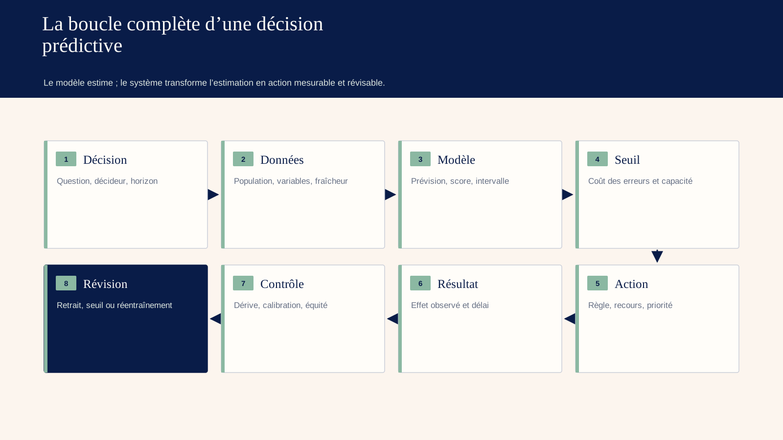
Predicting a delay does not reduce it. The system must choose who to alert, when, with what resource and error cost, and then check whether the action actually improves the result.
2. Key figures: more models, but no single universal method
- In France, 41% of companies using AI in 2024 used machine learning for data analysis, according to INSEE; more than one in two companies using AI combined at least two technologies.
- Eurostat measures that 20% of European enterprises with at least ten employees used AI technology in 2025, compared to 13.5% in 2024. This adoption increases the number of decisions potentially influenced by models.
- The M4 competition compared 61 methods on 100,000 time series. Of the 17 most accurate methods, 12 combined several approaches; the best hybrid reduced SMAPE by about 10% compared to the combination benchmark.
- The six "pure" machine learning methods of M4 obtained weak results, none exceeding the combination benchmark. This 2018 result does not condemn modern ML; it demonstrates the importance of baselines and ensembles on diverse data.
- The M5 then worked on 42,840 series sales hierarchies Walmart, illustrating an essential constraint: an item-by-item forecast must remain consistent with store, region and total.
- NIST AI RMF requires objective, repeatable or evolving testing, evaluation, verification and validation processes, as well as interpretation in the context of usage. A metric out of production is not enough.
The choice of method follows the data and the decision. The label "AI" does not confer any statistical advantage.
3. Decision table: nine columns before the first line of code
Build a table where each line represents an operational decision. The nine columns require the product to be defined, not just the target.
4. Column 1 — Decision and decision-maker
Write the action: order, recall, inspect, prioritise, set a stock level, trigger maintenance or investigate fraud. Name the person or team that uses the result.
"Predicting the demand" is too vague. "Recommend every Monday the quantity to be ordered for the next four weeks, under capacity and expiry constraints" defines a measurable use.
Check the timing. A forecast produced after the order, even if exact, has no value. The variables must exist before the decision point and the service must meet its deadline.
5. Column 2 — Current baseline
Document rule, intuition, simple model or lack of decision. Measure its performance and cost over the same period as the future system.
A seasonal average, last value, regression or trade score provides an indispensable reference. In M4, simple statistical combinations have surpassed several complex approaches; beating a credible baseline is more instructive than publishing a score without comparison.
Human baseline includes real capacity and information. An expert who receives ten files a day cannot be compared to a model classifying ten thousand cases without review constraints.
6. Column 3 — Outcome and time horizon
Define the target, unit, horizon, frequency and point at which ground truth becomes available. The 30-day default, the 12-week demand and the two-year customer value produce different learning patterns and cycles.
Avoid unvalidated proxies. A click does not replace a purchase, a lack of complaint does not prove satisfaction, and an unchecked case is not necessarily without fraud.
The truth can evolve after the fact: return, reimbursement, reopening or reclassification. Version the labels and define when a cohort becomes mature enough for evaluation.
7. Column 4 — Population and available data
Describe who or what receives a prediction, exclusions, coverage and sources at the exact time. Analyse missing, delayed, duplicated, censored or shaped by a previous policy.
7.1. Prevent data leakage
A variable created after the event, a code set by the investigator or an aggregation calculated on the future gives artificial performance. Training divisions must respect time, entities and groups.
In a forecast, use rolling validation: training on the past, testing on a future window, and then moving. A random split mixes seasons and may leave similar observations of the same series in both sets.
7.2. Understand selection bias
Confirmed frauds are based on controlled files, which have not been randomly selected. Clients who received an offer do not show what would have happened without an offer. The dataset reflects both historical policy and the phenomenon.
Document this mechanism and collect controlled exploration when it is ethical and possible.
8. Column 5 — Cost of errors and metrics
Accuracy, RMSE or AUC do not automatically translate the decision. Build the economic matrix of real/false positives and negatives, then choose the metrics that expose compromises.
8.1. Classification
Precision answers: among the alerts, how many are correct? Recall answers: among the real cases, how many are detected? AUC measures the ranking on all thresholds, but the workflow uses a specific threshold and a limited capacity.
If an event affects 1% of the population, predicting "no" everywhere offers 99% accuracy and zero utility. Publish confusion matrix, curves, performance at the threshold and absolute number of cases.
8.2. Forecasting
MAE describes an average absolute error, RMSE further punishes large deviations, MAPE becomes unstable near zero, and weighted metrics reflect commercial importance. Add bias, interval coverage and hierarchical consistency.
The correct metric remains understandable by the operator and related to a loss.
9. Column 6 — Probability, interval and calibration
A score of 0.8 should mean that about 80% of comparable cases occur, if use requires a probability. It can well rank and remain uncalibrated.
Reliability diagrams compare predicted probability and observed frequency per slice. The Brier score and log-loss are proper scoring rules, but the scikit-learn documentation reminds us that a lower Brier may reflect discrimination and uncertainty, not only better calibration.
For a forecast, provide quantiles or intervals. An inventory planner decides differently between 1,000 units with range 950–1,050 and the same average with 400–1,600.
Test calibration by segment and period. A correct average may hide a systematic overestimation among new customers or during promotions.
10. Column 7 — Action, threshold and capacity
The threshold comes from cost, capacity and recourse. If the team can review 200 files, the model must optimise the value of the first 200, not an overall metric.
10.1. Translate scores into actions
- below a threshold: standard treatment;
- intermediate area: information gathering or light intervention;
- above: priority action;
- out-of-distribution: abstention or expertise.
The threshold may vary by consequence, never by protected characteristic without legal analysis and non-discrimination. Any differentiation must have professional justification and control.
10.2. Separate prediction and prescription
A client at high risk of churn is not necessarily the one that a discount will save. Uplift modelling or experimentation seeks the heterogeneous effect of action; otherwise, the company can subsidize customers who would have stayed or irritate those who did not want to leave.
The shift from risk to intervention deserves its own causal evidence.
11. Column 8 — Integration and fallback options
The result comes in a tool, to a person, with context, explanation and delay. The interface shows useful factors without presenting a correlation as a cause.
The operator accepts, modifies or refuses and can report an incorrect data point. The corrections follow a process: they do not immediately retrain the model or become a truth without validation.
For decisions affecting individuals, organize information, challenge and review according to applicable law. An opaque score must not become an irreversible verdict.
12. Column 9 — Impact and retirement rule
First measure the technical performance on future data, then the impact of the decision. An experiment, progressive deployment or comparison of sites can estimate sales, delays, breakdowns, losses or modified satisfaction.
Pre-register thresholds: minimum gain, maximum error, tolerated disparity, cost, availability and load. Define withdrawal or fallback if an indicator breaks.
This estimate can remain accurate and lose its usefulness because price, capacity or strategy have changed. The withdrawal rule therefore relates to the complete business system.
13. Three predictive products, three different designs
13.1. Demand forecasting
The product delivers a distribution by item, place and horizon. It includes promotions, holidays, stockouts, prices, events and hierarchy. Replenishment optimisation adds storage costs, breakage, expiry and capacity.
The validation respects time and compares naïve seasonal, statistical method, ML and combination. The champion model can vary by segment; a robust set sometimes beats a unique architecture.
13.2. Risk scoring
The product ranks a population and calibrates a probability. It follows performance at the threshold, false positive/negative, stability, disparities, intervention and recourse.
The score does not replace policy. It feeds with an estimate whose use, period and limits are documented.
13.3. Anomaly detection
The product detects a deviation from a defined baseline. As anomalies are rare and changing, quality is judged on useful alerts, detection times, incident coverage and operator fatigue.
An unsupervised method detects unusual cases, not automatically fraud or breakdown. Human qualification and confirmed incidents are gradually creating a repository.
14. When a prediction score can destroy value
A chain of stores predicts seven-day demand every night and transmits the quantities directly to the replenishment engine. The average score improved by 8% compared to the baseline, but stockouts increased on key SKUs and stocks inflated on slow-moving products.
Diagnosis shows that the metric weighs each series almost equally, while the economics vary greatly: missing a traffic-driving product costs more than an identical error on a secondary reference, and overstocking a perishable item destroys more value than an additional unit of durable product.
The team therefore rebuilds the business loss with margin, break, substitution, expiration and space. It adds a constraint of consistency between article, category and store, then compares three order policies on a time backtest that reproduces the suppliers' timelines and limits.
Another mistake appears. Weeks with historical stockouts record low sales, which the model interprets as low demand; without availability indicator or censored demand estimate, the system learns to reduce precisely those items that had already been missed.
The patch is not just about changing the algorithm. The company improves the stock data, distinguishes observed demand and potential demand, sets a minimum stock level for some products and requires validation when the recommendation falls outside the training distribution.
Finally, a store-group trial compares the new policy with the existing resupply. Management follows net margin, availability, stock value, waste and intervention time, as a more accurate forecast justifies deployment only if the full decision produces a better compromise.
After eight weeks, the statistical error decreases less than expected, but availability increases by two points and waste decreases. The project succeeds thanks to a more faithful loss function, corrected data and limited policy, not due to the gross sophistication of the model.
The lesson goes beyond detail: any technical metric becomes dangerous when it ignores the asymmetry of consequences, the censoring created by the old policy and the constraints that transform prediction into action.
15. Quantified example: churn, propensity and uplift
One company has 100,000 clients, 10% of whom leave within three months. A churn model identifies 20,000 at-risk clients with a 30% churn rate: 6,000 churners, or 60% recall, and 14,000 false positives.
A discount of € 20 € is sent to the 20,000, maximum cost € 400,000 €. The starting rate drops to 24%, but without a control group it is not known how much would have remained or the effect on others.
A randomized trial on the eligible population then shows: 30% churn without the offer and 26% with it. The absolute lift is four points, 800 departures avoided out of 20,000; gross cost 500 € per customer saved if all discounts are consumed, before retention value.
The uplift analysis identifies a sub-group of 6,000 customers where the gap reaches twelve points. Treating only this group avoids about 720 departures for €120,000, or €167 gross per customer saved, while reducing the number of unnecessary discounts.
The figures are illustrative. They show that predicting risk, estimating effect and optimising decision are three distinct problems.
16. Monitor production: four drifts
16.1. Data drift
The input distributions change: new products, channels, formats or missing data. Compare the reference and qualify the impact, without warning on each benign variation.
16.2. Concept drift
The relationship between variables and outcome is evolving. A behaviour that previously predicted churn is no longer the case after a contract amendment.
16.3. Policy drift
The model changes actions, which change future data. Targeted investigation increases confirmed fraud in a segment, then the model learns that this segment is intrinsically more risky.
16.4. Value drift
Costs, prices, capacity or objectives are changing. The same score requires another threshold or no longer warrants intervention.
Monitor quality, calibration, volume, cost, segments, intervention and result. Plan for recalibration, retraining, revalidation or withdrawal depending on the diagnosis.
17. Predictive-service architecture
- data contracts and quality;
- calculated features with correct temporality;
- dataset/version/lineage;
- repeatable training;
- model register and approval;
- Batch or API with SLA;
- rules, thresholds and business capacity;
- interface and recourse;
- technical, statistical and economic monitoring;
- fallback to baseline.
Fallback is a built-in feature. If the day's data is missing, the decision must revert to a safe rule.
18. Logiks twelve-week programme
18.1. Weeks 1 to 3 — Decision framework and baseline
Define action, population, horizon, costs, capacity and current rule. Audit the temporality of the data.
18.2. Weeks 4 to 6 — Backtest and calibration
Build time splits, compare baselines and models, evaluate segments, probabilities and intervals. Document errors.
18.3. Weeks 7 to 9 — Shadow mode
Produce scores without changing the decision. Check time, coverage, interface and stability on truly unseen future data.
18.4. Weeks 10 to 12 — Controlled impact
Open action on a perimeter, measure result and cost, maintain control or comparison. Decide whether net value justifies scaling.
This calendar is a Logiks example. The maturity of the labels, seasonality and horizon may require several months.
19. Logiks recommendations: twelve classic traps
- choosing accuracy for a rare event;
- using a future variable;
- randomising a time series;
- treating stockouts as ordinary zeros;
- confusing score and probability;
- ignore intervals;
- optimising AUC without operational capability;
- treat risk as an effect of action;
- reusing the decisions of the model without exploration;
- explaining correlation as a cause;
- monitor features without monitoring the value;
- keeping a model because it cost a lot.
Any model remains a deployed hypothesis. It remains revocable.
20. FAQ
20.1. What is the difference between forecasting and prediction?
Forecasts often focus on a future value indexed over time; prediction includes classes, scores and unknown states. Both require out-of-sample validation.
20.2. Which algorithm should you choose?
Compare baseline, statistical methods, trees, networks or combinations on your data, horizon, cost and constraints. The most precise is not always the most useful.
20.3. AUC or accuracy?
Neither one of them alone. Use precision, recall, the confusion matrix, calibration, threshold performance and expected value depending on the problem.
20.4. How do I detect drift?
Monitor entries, results, calibration, residuals, segments, actions and economics. A variation in distribution does not always imply a loss of usefulness.
20.5. Should we explain every prediction?
The level depends on the risk and use. The operator needs an actionable context, the governance team needs overall validation, the affected person needs appropriate information and redress.
20.6. When should you retire a model?
When it no longer beats the baseline, exceeds errors or disparities, costs more than its value, cannot be maintained or no longer corresponds to the decision.
21. Conclusion
Predictive AI does not transform the data into certainty. It turns uncertainty into an estimate, and then the company decides whether this estimate deserves action.
Define the decision. Respect temporal order. Compare a baseline. Calibrate probabilities. Separate prediction and causality. Finally measure the impact and keep a way back.
The value appears after the score.
22. Main sources
- Insee, Artificial Intelligence in Enterprises, 14 October 2025: https://www.insee.fr/fr/statistiques/8616837
- Eurostat, 20% of EU enterprises use AI technologies, 11 December 2025: https://ec.europa.eu/eurostat/web/products-eurostat-news/w/ddn-20251211-2
- Makridakis, Spiliotis and Assimakopoulos, The M4 Competition: 100,000 time series and 61 forecasting methods, International Journal of Forecasting: https://www.sciencedirect.com/science/article/pii/S0169207019301128
- Google Research, The M4 Forecasting Competition — A Practitioners View: https://research.google/pubs/the-m4-forecasting-competition-a-practitioners-view/
- Makridakis et al., M5 accuracy competition, data from 42,840 series: https://www.sciencedirect.com/science/article/pii/S0169207021001874
- NIST, AI RMF Core - Measure: https://airc.nist.gov/airmf-resources/airmf/5-sec-core/
- scikit-learn, Probability calibration: https://scikit-learn.org/stable/modules/calibration.html